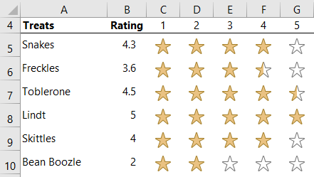
Creating an Excel five star rating chart is easy with Conditional Formatting. They’re not limited to stars, you can also create column, pie and waffle rating charts.
Constructing an Excel Five Star Rating Chart
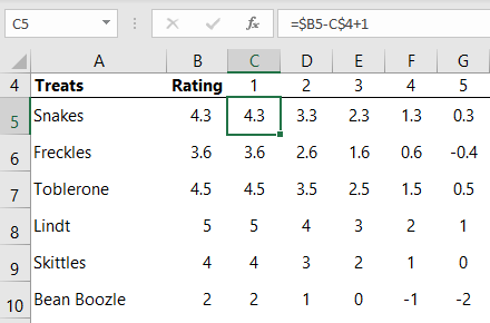
Step 1: In the top left cell of your table, in my case cell C5, insert the formula below that calculates the portion of star for each column; 1 through 5:
=$B5-C$4+1
Tip: If you’re using Office 365* you can use the following Dynamic Array formula instead, which means you don't need the numbers 1-5 in row 4:
=$B5-SEQUENCE(1,5)+1
More on the SEQUENCE function here.
*At the time of writing, Dynamic Arrays are only available in Office 365 and are currently in beta on the Insiders channel. Excel 2019 will not have the Dynamic Array functions.
Step 2: Copy the formula in C5 to all cells in the table, i.e. C5:G10. It returns the following results:
Step 3: Set the Conditional Formatting to apply a whole star to any value that is greater than or equal to 1.
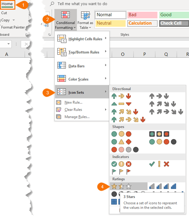
Make the following selections in the Conditional Formatting dialog box:
Tip: If you don’t want the empty star to show you can set the < 0.5 star to ‘No Cell Icon’:
And now you have an Excel five star rating chart:
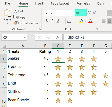
Tip: Set the cell font size to alter the size of the stars to suit and hide the 1 – 5 numbers in C4:G4 by formatting them in a white font.
Other Excel Rating Charts
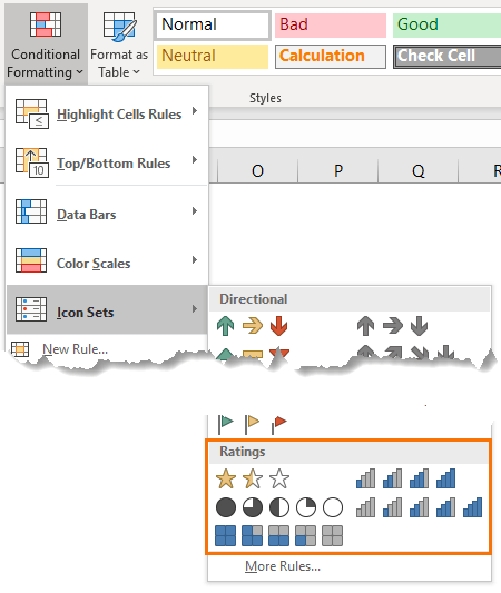
You’re not limited to star ratings. Conditional Formatting icons also have pies, column charts and waffle style charts:
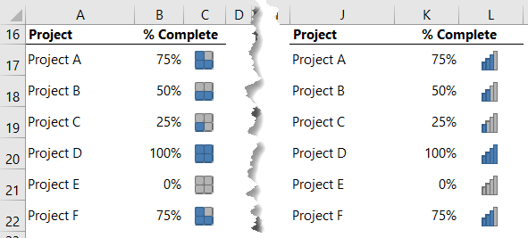
Examples of the waffle and column charts are below and included in the Excel file for download below:
Download Workbook
Enter your email address below to download the sample workbook.
Related Lessons
How to use Conditional Formatting
Conditional Formatting Excel Heat Maps
The mystery behind Conditional Formatting Formula Based Rules
Conditional Formatting Gantt Chart
Conditional Formatting in PivotTables
Toggle Conditional Formatting On and Off
Please Share
If you liked this please share this tutorial with your friends and colleagues.

Elegant work, as usual.
If you are going for a spilt array why not go for a 2D array formula
= Rating – SEQUENCE(1,5,0)
and take a step towards eliminating relative referencing?
Hi Peter,
Thanks for your kind words. I did suggest using SEQUENCE in the ‘tip’ under Step 1. Albeit I used SEQUENCE(1,5)+1.
Mynda
I did see you formula. That’s what prompted me to try ‘Rating’
= $B$5:$B$10
and watch the 2D spill to cover all the treats with one formula.
( In reality I was an opportunity to play with the new array toys! 🙂 )
Ah, it was the range information for ‘Rating’ I was missing 🙂 The dynamic arrays sure are fun!
When I put the formula =$B2-C$4+1 into the grid it return a number 1 in every rating, what am I doing wrong?
Hi Boni,
Are there any values in cells B2 and C4 in your worksheet? If these cells are empty or zero the formula will return 1.
Mynda
It would be good if the color of the stars can change depending on its number.
I would normally use Wingdings font together with conditional formatting to achieve this effect.
Another method is to use the REPT function. Both method uses CHAR(171) for the full star and CHAR(182) for the half star.
Good to know there are so many methods to achieve the same result in Excel
Thanks for sharing, Sunny. I like the conditional formatting option too.