The Excel MATCH function looks up a value in a range and returns the relative position of that value.
The range can take the shape of a row or column. On its own the MATCH function isn't very exciting, but it's super useful when nested with INDEX and VLOOKUP etc.
Excel MATCH Function Syntax
| Syntax: | =MATCH(lookup_value, lookup_array, [match_type]) |
Excel MATCH Function Arguments
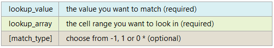
*The match_type behaviour varies depending on the setting as described below.
| match_type | Behaviour |
| 1 or omitted | MATCH finds the largest value that is less than or equal to lookup_value. The lookup_array values must be sorted in ascending order. |
| 0 | MATCH finds the first exact value that is equal to lookup_value. The values in the lookup_array range don't need to be sorted. |
| -1 | MATCH finds the smallest value that is greater than or equal to lookup_value. The lookup_array values must be sorted in descending order. |
Download the Workbook
Enter your email address below to download the sample workbook.
Excel MATCH Function Text Examples

Excel MATCH Function Notes
- MATCH returns the position of the matched value within the 'lookup_array', not the value itself.
- MATCH is not case sensitive when matching text values. See example on row 6.
- When using the 'match_type' 0, MATCH will return the #N/A error value if it is unsuccessful in finding a match. See example on row 9:
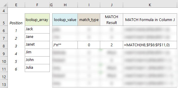
- Wildcard characters like the question mark (?) and asterisk (*) can be used in the 'lookup_value' argument when the 'match_type' is 0 and the 'lookup_value' is a text string. A question mark matches any single character; an asterisk matches any sequence of characters. If you want to find an actual question mark or asterisk, type a tilde (~) before the character. See examples on rows 7 and 8.
- If the 'lookup_array' contains duplicates of the 'lookup_value', MATCH will return the position of the first occurrence. See example on row 8 where J*n** could be Jane or Janet and MATCH returns the position of the first match, which is Jane.
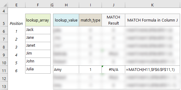
- When using ‘match_type’ 1, MATCH will return an error if the ‘lookup_value’ is smaller than the smallest value in the ‘lookup_array’. See example on row 11 where Amy is ‘alphabetically’ smaller than any of the values in the ‘lookup_array’.
- When using ‘match_type’ -1, MATCH will return an error if the ‘lookup_value’ is larger than the largest value in the ‘lookup_array’. See example on row 12 where Robert is ‘alphabetically’ larger than any of the values in the ‘lookup_array’.


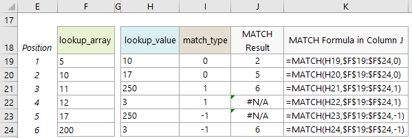
Excel MATCH Function Numeric Examples
Excel MATCH Function - Find Largest Value
So, now we know that ‘match_type’ argument 1 finds the largest value that is less than or equal to lookup_value, we can exploit this rule to find the position of the largest value in a range.
All we need to do is enter a really big number as the ‘lookup_value’ argument. A value so big it will never be found in the ‘lookup_array’. For example, 1E+10 is the scientific notation for 10,000,000,000. If you think your ‘lookup_array’ could have numbers bigger than that, you can use 1E+100.
The formula below can be used as a template for finding the location of the biggest number in your ‘lookup_array’. Simply replace ‘lookup_array’ with the range of cells you want to check:
=MATCH( 1E+100, lookup_array, 1)
Note: The ‘lookup_array’ must be sorted in ascending order.
Tip: If you want to return the actual number, as opposed to the position, you can use INDEX and MATCH like this:
=INDEX(lookup_array, MATCH( 1E+100, lookup_array, 1) )
Excel MATCH Function - Find Smallest Value
Likewise, we can use the ‘match_type’ argument -1 to find the position of the smallest value.
=MATCH( -1E+10, lookup_array, -1)
Note: The ‘lookup_array’ must be sorted in descending order.
Tip: Again, if you want to return the actual number, as opposed to the position, you can use INDEX and MATCH like this:
=INDEX(lookup_array, MATCH( -1E+100, lookup_array, -1) )
Related Functions
| INDEX Function | The Excel INDEX function can lookup a range of cells and return a single value, an array of values, a reference to a cell or a reference to a range of cells. |
| VLOOKUP Function | The VLOOKUP function looks up a value in a column and returns a corresponding value from a column to the right. |
| HLOOKUP Function | The HLOOKUP function looks up a value in a row and returns a corresponding value from a row below. |
Excel MATCH Function Formula Examples
Excel Factor Entry 4 INDEX and MATCH Two Criteria
Return the First and Last Values in a Range