At first glance the CHOOSE function isn’t very exciting and typically you have to team it up with other functions to get the party started. Fair enough I suppose, after all, the more the merrier.
In this tutorial we’re going to use choose to toggle through different aggregation methods (AVERAGE, MAX, MIN, SUM) as seen here:
Download the Workbook
Enter your email address below to download the sample workbook.
CHOOSE Function
But first a quick rundown for those not familiar with CHOOSE:
The syntax is:
CHOOSE(index_num, value1, [value2], [value3],….)
It returns a value from a list based on the index_num argument.
A simple example:
=CHOOSE(2, "Functions","PivotTables","Macros","Tables")
Would return PivotTables as it’s the second value in the list.
Whereas
=CHOOSE(4, "Functions","PivotTables","Macros","Tables")
Would return Tables because the index_num argument is 4, and Tables is the 4th value.
One of the unique features of CHOOSE is that the value arguments can be:
- Numbers
- Cell references
- Defined names
- Formulas
- Functions
- Text (as in the above examples)
CHOOSE Party
That’ a long list of options and provides a huge range of applications (and opportunities to party...sorry, I couldn't help myself ;-)).
There are a few moving parts to this technique:
Is your head in a spin? Let me explain them:
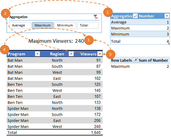
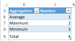
- CHOOSE's index_num argument comes from a Table called agg that maps the aggregation type to the index number:

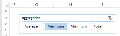
- Slicers (available in Excel 2010 onwards) provide the interactivity that enables the user to toggle through the different aggregation methods:
- The Slicer filters a mini PivotTable (mini being small and with the Grand Total line removed, as opposed to some special breed of PivotTable):
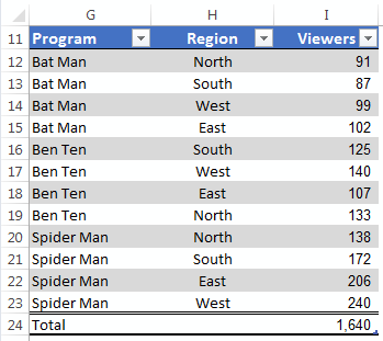
- Our data is formatted in an Excel Table called ProgramTbl2 (see below) and this means our formula will be using Structured References to reference the table.
- And our CHOOSE formula in cell I9 references cell L13 of the PivotTable to find which aggregation method was selected:
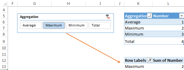
=CHOOSE(L13, AVERAGE(ProgramTbl2[Viewers]), MAX(ProgramTbl2[Viewers]), MIN(ProgramTbl2[Viewers]), SUM(ProgramTbl2[Viewers]),)
Bonus: in cell H9 there is a dynamic text label which also uses CHOOSE to display which aggregation method has been chosen:
=CHOOSE(L13,"Average","Maximum","Minimum","Total")&" Viewers:"
Excel 2007 Method
For those of you still using Excel 2007 you don’t have the luxury of Slicers but you can achieve the same results using Form Control Radio Buttons:
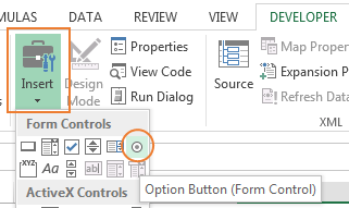
- To insert radio buttons you first need to enable the Developer tab in your Ribbon.
- After selecting the Radio Button from the Insert drop down on the Developer tab simply left click and drag the mouse to draw it on your workbook. Right-click it to edit the text.
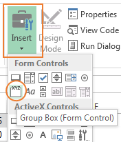
- Make sure you put them in a Group box (Form Control) so Excel knows they’re all part of a group and numbers them consecutively. Click and drag to draw the Group Box on your worksheet just like you do with the Radio Buttons.
Tip: the whole of each Radio Button must be inside the bounds of the Group Box.
- Set the Cell Link cell for each Radio Button. Right-click the Radio Button > Format Control > Control tab and choose a cell for the Cell Link (mine is in cell E7):
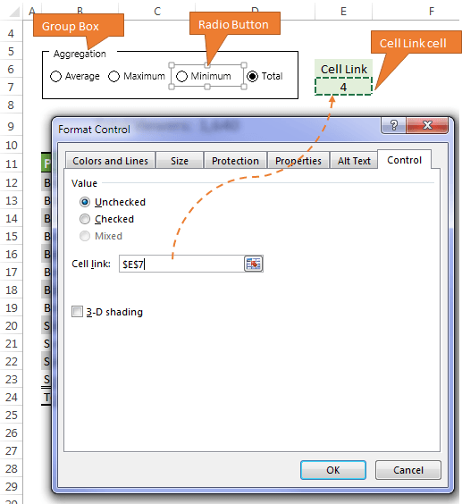
The Cell Link is a cell anywhere in your workbook which captures the number of the selected radio button. All 4 of your radio buttons should use the same cell as this populates the index_num argument in your CHOOSE formula.
Note: you’d normally put your Cell Link cell out of sight. I put beside the radio buttons so you can see all the moving parts together.
Tip: you can copy and paste the first Radio Button and it will remember the cell link so you only have to set the Cell Link once.
- Link your index_num argument to the Cell Link cell.
=CHOOSE(E7,AVERAGE(ProgramTbl[Viewers]),MAX(ProgramTbl[Viewers]),MIN(ProgramTbl[Viewers]),SUM(ProgramTbl[Viewers]))
Toggle away!
Uses for this technique
- Headline figures in your Dashboard reports
- A quick way to summarise your data in different ways
- Use it with named ranges to return different regions/product group summaries
More CHOOSE Examples
- A fairly common way to use CHOOSE is to force VLOOKUP to look to the left. Although I prefer INDEX & MATCH for this.
- Mike Alexander shows us a clever way to use CHOOSE to convert a date into a fiscal quarter.
Totals in Excel Tables
Excel Tables also enable you to choose the aggregation method by clicking on the down arrow in the Total cell:
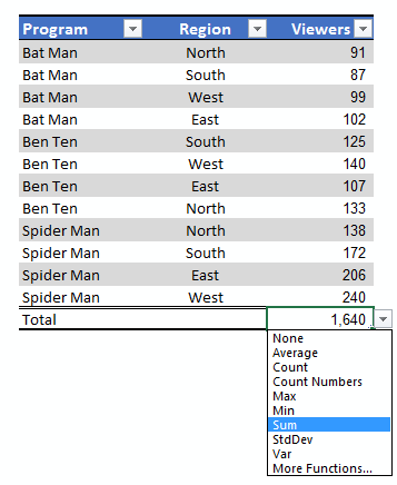
It’s a nice touch, however there are two things I don’t like about this:
- The ‘Total’ label in the first column doesn’t change to tell you what aggregation method is in use. You can choose Standard Deviation and ‘Total’ still says ‘Total’.
- It’s at the bottom of the Table which can be a long way away.

I know this is a Choose exercise but another solution is to do it simpler and yet more versatile.
Enter the following.
C26 Analysis D26 Viewer Stats
C27 Average D27 =AVERAGE(ProgramTbl[Viewers])
C28 Maximum D28 =MAX(ProgramTbl[Viewers])
C29 Minimum D29 =MIN(ProgramTbl[Viewers])
C30 Total D30 =SUM(ProgramTbl[Viewers])
Now convert this to a table and any or all of the Statistics can be selected or visible.
The table can be dragged elsewhere, say above the ProgramTbl table as Jonathan likes, or even to another sheet.
Regards,
Ru
Regards your comments about “there are (two) things I don’t like about thi ……The total’ still says ‘Total’. It’s at the bottom of the Table which can be a long way away.”
Whenever I insert a table I always activate the Totals row. It might in Row 1217 for all I know.
I then insert a row above my table headers In Row1 so now I have a clean row of white space immediately above my Table Headers.
I then click in a column heading cell in Row1, (example Cell G1), type an = and then click in the cell containing the Totals value at the bottom of the table column.(example Cell G1217) This now shows the Total value at the bottom AND the top of the table. Repeat for all other totals that you want to see at the top above your headings. I find because they are dynamic they are fantastically more convenient than having to continually trawl to the base of the table.
Thanks for sharing your approach, Jonathan.
ciao Mynda!
I quickly looked at your file … and I immediately thought of a different solution …
chenge pivot table value in:
Aggregation Number
Average 1
Maximum 4
Minimum 5
Total 9
then in I9 =SUBTOTAL(L13,ProgramTbl2[Viewers])
ummm … end in H9 i think we can write =K13&” Viewers:”
I take this opportunity for a big CIAO to you
🙂
regards
r
CIAO to you too, Roberto. Lovely to hear from you.
Thanks for your idea. I also thought about using AGGREGATE but that wouldn’t demonstrate CHOOSE 😉 nor would it work in Excel 2007 with radio buttons.
Mynda
First of all, I want to say thank you for all the wonderful tips you put out!
I like the thought behind this tip. I noticed one thing that a person has to watch out for. Since by design, slicers allow a person to make one or multiple choices, a person may do that in another scenario with different data where it would be appropriate to make several choices at once, but using this slicer method only one of them will show.
So, visually, if two choices are made via the slicer – it is fine if one looks strictly at the heading, but if one is thinking of what choices he made or visually looks at the slicer (and not the heading), he will be getting the wrong impression of what the data is representing.
Good point, Paul. Thankfully in Excel 2016 you can set a Slicer to only use single selection, but in earlier versions you’d have to write error handling into your formula to tell them they can’t pick multiple items.
I’m running Office 2016 and dabbled with the Multi-Select option in the slicers. This just seems to be a way to allow a user to select multiple items without knowing about CTRL or SHIFT as selection controls. The user can still select multiple items via the keyboard.
Below is a macro that will detect the selection of multiple items in a slicer and reject all of them except for one. Paste this into the code window of the sheet that contains the slicer.
I used the name of the table and slicer that Mynda used in her example file:
Pivot Table Name: PivotTable1
Slicer Name: Aggregation
In the immortal words of the Sirius Cybernetics Corporation:
“Share and Enjoy!”
=============================================
Private Sub Worksheet_PivotTableUpdate(ByVal Target As PivotTable)
Const CONTROL_PIVOT As String = “PivotTable1”
Const CONTROL_FIELD As String = “Aggregation”
Dim pi As PivotItem
Dim itemFound As Boolean
On Error GoTo wp_exit
Application.EnableEvents = False
If Target.Name = CONTROL_PIVOT Then
With Target.PivotFields(CONTROL_FIELD)
For Each pi In .PivotItems
If pi.Visible Then
If itemFound Then
pi.Visible = False
Else
itemFound = True
End If
End If
Next pi
End With
End If
wp_exit:
Application.EnableEvents = True
End Sub
Brilliant! Thanks for sharing, Bryon 🙂
Mynda