I’ve always thought after inserting a PivotTable that Excel should ask “would you like a PivotChart with that?”. I think PivotCharts are Microsoft’s equivalent of McDonald’s famous upsell – “Would you like fries with that?”
I’m not saying you should have Excel Pivot Charts with every PivotTable meal but they do go nicely together. However, beware; PivotCharts have their own set of rules which you must abide by, and for that reason they come with a health warning!
And if Pivot Charts are the equivalent of fries then Slicers are the ketchup – you can have them with your PivotTable and or Pivot Charts. More on Slicers in a moment.
Download the Workbook
Enter your email address below to download the sample workbook.
Watch the Video
Be sure to watch till the end to see my blooper 🙂
Inserting a Pivot Chart
In Excel Pivot Charts can be inserted without first creating a PivotTable. You’ll find them on the Insert tab. In Excel 2007/2010 they're in the Tables group and in Excel 2013 you'll find them in the Charts group:

The drop down gives you the option to either insert a PivotChart or Insert a PivotChart & PivotTable, which appears to be superfluous* since either option opens the menu you’re probably familiar with (notice the only difference is one says ‘PivotTable’ and the other says ‘PivotChart’):
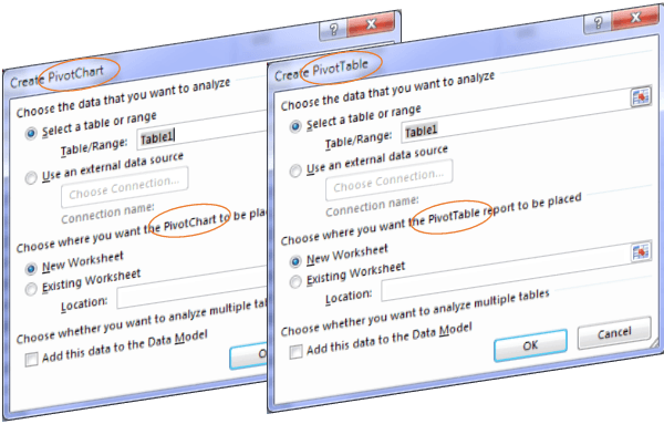
And when you’ve selected your data and where you want to place the PivotChart, or PivotTable & PivotChart, you’ll have an empty PivotTable and PivotChart (irrespective of whether you choose to insert just a PivotChart), and the field list is open ready for you to build your chart and table:
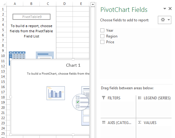
Notice how with the PivotChart selected the Field List (above) has a Legend (Series) and Axis (Categories) sections instead of the usual Columns and Rows for a PivotTable. Nice touch.
*Note: it is only possible to insert a PivotChart without a PivotTable in Excel 2013 if you check the 'Add this data to the Data Model' check box upon inserting the PivotChart. But then you're working in Power Pivot and that has its own implications, which is for another day.
Adding a PivotChart Later
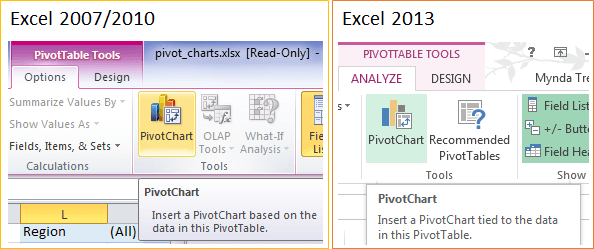
Sometimes we build the PivotTable and then decide to add a PivotChart. You’ll find the option on the PivotTable Tools: Analyze/Options tab (when the PivotTable is selected).
Switch Rows/Columns
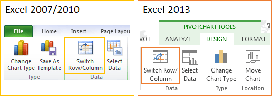
When you insert a chart you might find that you need to change the location of the rows and column labels to better suit the layout of the chart. If so you can either go back to the field list and switch them or right-click the chart > Select Data > Switch Row/Columns, or on the PivotChart Tools: Design Tab > Switch Row/Columns.
Changing the Chart Type
You can change the chart type by right-clicking on the PivotChart > Change Chart Type or on the PivotChart Tools: Design menu (see image above).
PivotChart Limitations
PivotTables are fussy; they only let you use their data in a PivotChart, i.e. you can't insert any old chart from the Insert Chart menu. In fact you can’t insert an XY Scatter, Bubble or Stock chart with your PivotTable data.
PivotCharts are all or nothing; one of the most common questions I get asked is ‘how can I only display some of the data from the PivotTable in the chart?’ The answer is you can’t pick and choose which data in the PivotTable is displayed in your chart. It’s all or nothing, with the exception of Grand Totals which are not displayed in your charts.
Field Buttons and Slicers
Once you’ve built your PivotChart you’ll find there are Field Buttons on the chart.
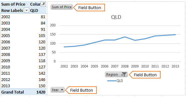
The buttons with a drop down arrow are interactive and you can use them to change the filters and sort options, which is pretty powerful:
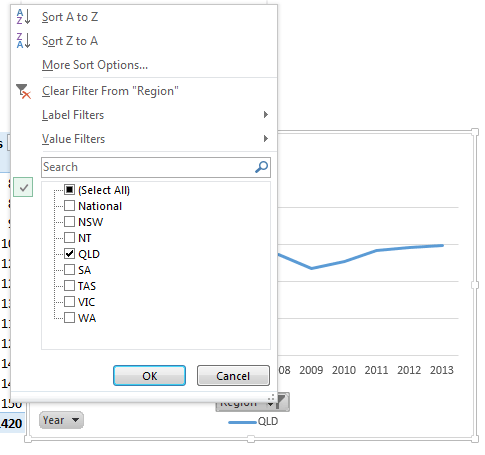
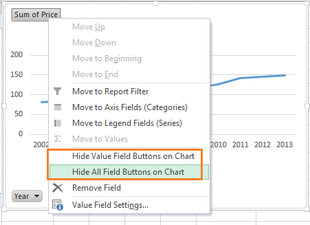
However, I prefer to use Slicers for filtering as the Field Buttons are space hogs and you can't customise them, or their location. To remove them right-click any of the Field Buttons > choose to either Hide All or Hide Value Field Buttons:
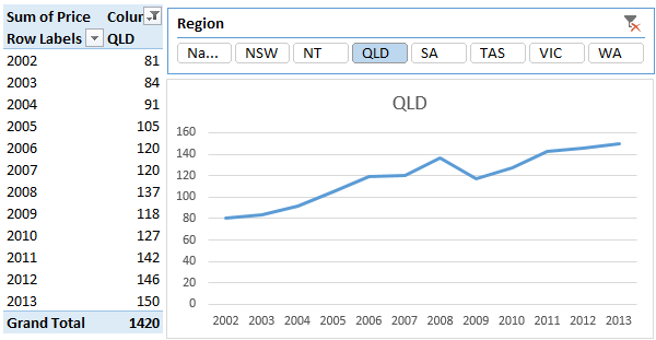
Slicers
If you have Excel 2010 or later you can use Slicers instead of the Field buttons for a more intuitive interface.
It wasn’t a blooper it was sweet/cute.
Hey Maynda,
I have created Dashboard in excel with different charts table , but I got face one thing when I click on any charts he show with his property I don’t want to need this i want to locked or fixed this charts
Hi Nabeel,
I don’t understand the issue.
Can you please start a topic on the forum and supply your workbook.
Regards
Phil
Mynda, how can I make a dynamic chart title on a pivot chart that is based on the filtered field?
Hi Bill,
This would only be feasible if there is only likely to be between 1 and 3 items selected in your Slicer. Anymore than that and your chart title will be too long.
If so, then in a cell in your worksheet you build a formula that picks up the rows visible in your PivotTable and concatenates them. These visible rows contain the items selected in your Slicer. You can then link the chart title to the cell containing your concatenation formula.
These tutorials go into more detail:
https://www.myonlinetraininghub.com/excel-dynamic-text-labels
https://www.myonlinetraininghub.com/excel-textjoin-function
If you get stuck please post your question on our Excel Forum and a sample Excel file so we can help you in more detail.
Mynda
Thank you for sharing your knowledge of Excel! All these tools and tips are very helpful for better presentation of data.
You’re welcome, Maryam. I’m glad you find them useful.
Mynda
Thanks for all your tips.
Great to know you like them, Anne 🙂
Hi Mynda,
how to add Field Buttons on Chart.
I use 2007
Thanks & kind regards
Raghu
Hi Raghu,
In Excel 2007 you don’t have the Field buttons on the chart. Instead you have a PivotChart Filter Pane which hovers above your worksheet. You can turn it on by selecting the PivotChart and then on the PivotChart Tools: Analyze tab select ‘PivotChart Filter’.
I hope that helps.
Kind regards,
Mynda
As usual, some really helpful information. Your website and courses are easy to follow and very clear. Thank you.
Thanks, Suz 🙂
Hi, I love your site and all of the Excel tips you give. When I tried to download the workbook it did not work. Thanks!
Hi Michael,
Thanks for your kind words.
Sorry about the workbook download link, I’ve fixed it now. Here is the correct link
Kind regards,
Mynda