Excel PivotTable Calculated Items

Inserting Excel PivotTable Calculated Items is a great way to analyse your data and automatically incorporate that analysis in your PivotTables.

Another way to think of them is the ability to add a new item to your report based on a formula which uses other items in the column. You can then include this new item in any PivotTable report, as though it were part of your source data.

Download the Workbook

Enter your email address below to download the sample workbook.

By submitting your email address you agree that we can email you our Excel newsletter.

Please enter a valid email address.

Download the Excel Workbook. Note: This is a .xlsx file please ensure your browser doesn't change the file extension on download.

Watch the Video

Visualising a Calculated Item

I like to differentiate a Calculated Field from a Calculated Item by picturing where they would appear if they were part of your source data:

PivotTable Calculated Fields are the same as columns in your source data

PivotTable calculated fields

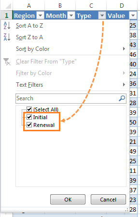
PivotTable Calculated Items are the same as the different items inside those columns, or another way to think of them is to imagine they are the same as the items you see in the list when you click on the filter drop down buttons.

PivotTable calculated items

Inserting Calculated Items

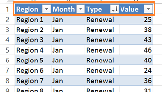
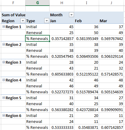
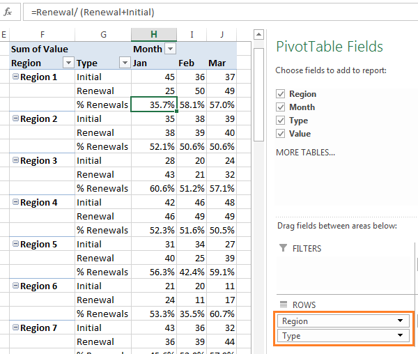
The PivotTable below contains sales by region split by Type: Initial Sales and Renewal Sales. We’ll add a Calculated Item for the percentage Renewal Sales are of the total sales.

PivotTable calculated item example data

The first thing you must do is select a cell in the PivotTable rows or columns area (i.e. any of the cells not containing numbers), and if you choose a cell in the row/column where you want your item added it’ll save you a step. We’re adding a new Type so I’ll select any cell in column G of the PivotTable.

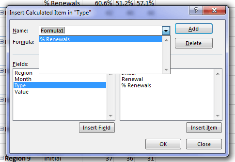
Then on the PivotTable Options tab (Excel 2010), or PivotTable Analyze tab (Excel 2013) > Fields, Items & Sets > Calculated Item. This opens the dialog box below:

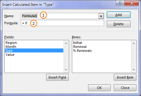
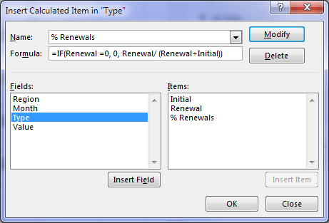
Insert PivotTable calculated item

Give my new Item a name. I’ll call it % Renewals
My formula for % Renewals will be:

= IF(Renewal=0, 0, Renewal / (Initial + Renewal))

Translated to English reads: IF the Renewal value = 0, then return zero, otherwise calculate Renewal divided by the sum of Initial + Renewal.

The reason I added the IF is to avoid any #DIV! errors should the Renewal value ever be zero.

In the Insert Calculated Item dialog box my formula it looks like this:

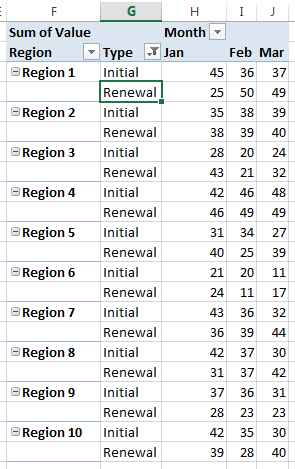
Insert PivotTable calculated item

When you add the new Calculated Item it’s automatically included in your PivotTable:

Insert PivotTable calculated item result

Formatting Calculated Items

Now we have a dilemma; we need the % renewals formatted with the percentage sign but applying a number format to the field (via the Value Field Settings menu) would mean all values are displayed as a %, so instead we need to apply the formatting just to the cells for the % renewals. Don't forget to make sure the ‘Preserve cell formatting on refresh’ is checked.

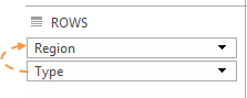
The quickest way to do this is to switch the order for Region and Type so all the Types are grouped together. Simply drag Type above Region in the field list:

Switch PivotTable rows order

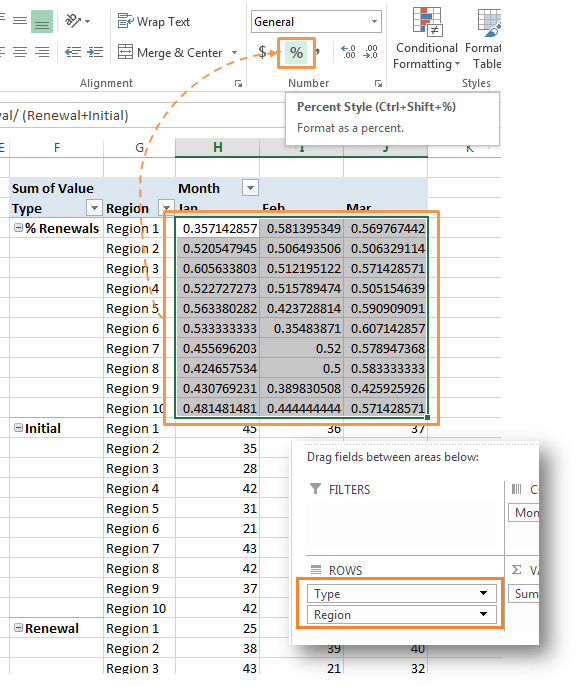
Then we can select all the cells we want to format and apply the formatting using the Format Cells menu on the Home tab, or CTRL+SHIFT+%:

Format PivotTable calculated item

Then you can switch your Region and Type columns back and the formatting sticks:

Formating sticks

Tip: notice in the formula bar that the formula for the calculated item is visible. You can also edit this formula just as you would any other, but beware, it will only edit it for the active cell and all other formulas will remain as they were.

Calculated Item Formula Rules

Above is just one example of inserting a calculated item, however applying the rules below will open up many more uses for them:

Operators: you can use operators and expressions as you do in other worksheet formulas (+ - * / ^ < >).

Constants: you can use constants and refer to data from the report, but you cannot use cell references or defined names.

Functions: you can’t use worksheet functions that require cell references or defined names as arguments, and you can’t use array functions.

Not compatible with OLAP PivotTables - You can only insert calculated items in PivotTables created with non-OLAP data sources. For most of us that’s ok since data in an Excel worksheet is a non-OLAP data source.

Calculated Items Example 2 – Reconciling

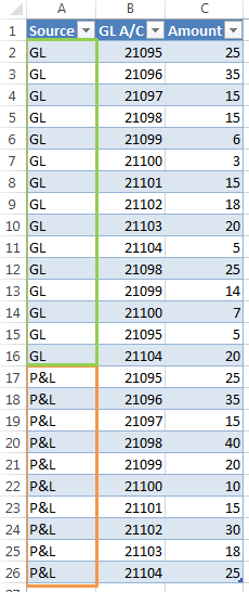
Last week I was asked if there was an easy way to reconcile a General Ledger to a P&L. The answer is yes, a PivotTable is a great tool to use. Let’s take a look; here is our data which contains the amounts by GL Account for two sources: the General Ledger (GL) and the P&L:

calculated item for reconciling

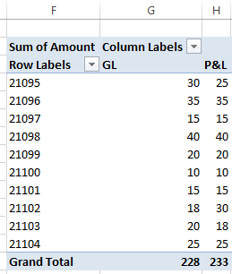
I’ll insert a PivotTable that summarises the Amounts by GL Account and then we can compare the GL balances to the P&L balances:

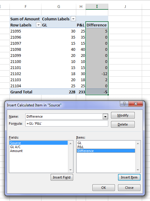
calculated item for reconciling accounts

Now I can insert a calculated item (called Difference) to subtract P&L from GL:

calculated item for reconciling account differences

Modifying and Deleting Calculated Items

If you want to edit or delete a calculated item simply go back to the PivotTable Options/Analyze menu > Insert Calculated Item > click on the drop down list in the Name field and select the item you want to delete or edit:

modify calculated items

From here you can make your changes to the formula or click the ‘Delete’ button to get rid of it altogether.

Referencing Items by Position

Another way you can reference items in the formula is by their position in the PivotTable. For example, GL is the first item and P&L is the second, therefore we could write the formula like this:

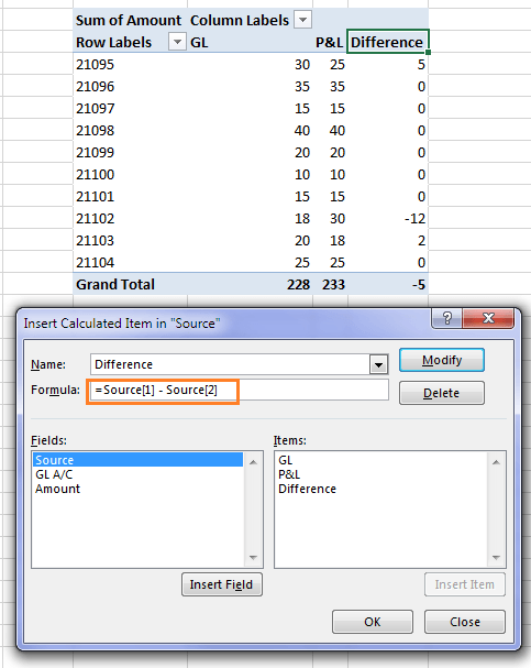
reference calculated items by position

Items referred to in this way can change whenever the positions of items change or different items are displayed or hidden. Note: hidden items are not counted in this index.

For example, if you moved the order of the items through sorting, P&L could become Source[1] and GL could become Source[2].

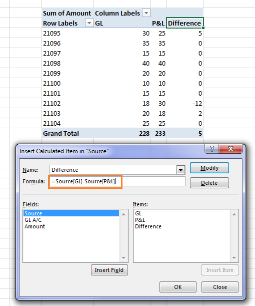
Referencing by field name

And in the event that there might be a name conflict (caused by items in different fields having the same name) resulting in #NAME? errors, you can reference the items by their field and item name like so:

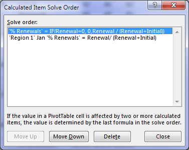
reference calculated items by field names

Calculated Items Solve Order

If you have multiple calculated items you can alter the order in which they are calculated by rearranging the Solve Order (PivotTable tools > Options/Analyze > Solve Order):

change solve order of calculated items

Calculated Item Gotchas

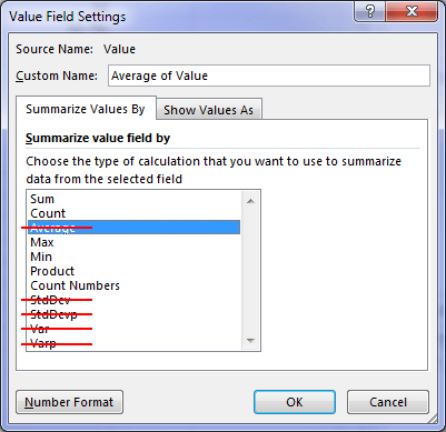
Unfortunately once you insert a calculated item into your PivotTable you can no longer summarise your values by Average, Standard Deviation or Variances 🙁