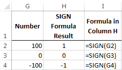
The Excel SIGN function returns a 1 if the number is positive, a zero if it’s zero and a -1 if the number is negative.
The syntax is simple: =SIGN(number)
Here are some basic examples:
So what’s it good for?
Well, last week we had a request for help from Alston. He was comparing the variances for Actual vs Forecast year on year.
This reminds me of my accounting days where one of my monthly tasks was to produce Actual Cost vs Budget/Forecast Cost reports.
Aside: Variances are calculated as =(Budget - Actual).
Our reporting standard was to present negative figures in brackets, and to pre-empt the question I received regularly from the department heads (who weren't finance people); "are negative variances good or bad?" I had a chant “remember, brackets are bad news” :-).

For my North American friends, brackets are the same as parentheses but saying “parentheses are bad news” just doesn’t have the same ring to it.
Occasionally I’d also throw in a “c’mon, Finance is Fun” line when I saw them frowning as I approached their office.

I’m pretty sure they laughed at me rather than with me, but at least they were smiling as I slipped the report on their desk (printing was big back then), or chased them up for their forecast figures, or requested an explanation for why they were 50% over budget and it was only March! 🙂
Ah, those were the days.
Excel SIGN Function Example
Let’s look at a clever use for the SIGN function which is along the lines of Alston’s question; here is a table of dummy variance data (Actual Cost vs Budget Cost variances) for 2013 and 2014 by department:
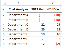
Note: For the purpose of this we’ll assume that the budgeted figures for 2013 and 2014 are the same for each department so we can focus on comparing the change in variances.
With some high school math we can calculate the percentage change in variance for department A like so:
=(C2-B2)/B2)
=(-10 - -18)/-18)
=8/-18
=-44%
The problem here is the 2014 negative variance is lower than the 2013 negative variance so this should be an improvement year on year of 44% but the percentage is calculated as -44%.
Unfortunately it's not as simple as reversing the formula to subtract B2 - C2 etc. either.
So, in struts the SIGN function to the rescue:
=(C2-B2)/B2*SIGN(B2)
=44%
If we look at the other departments we can see the SIGN function returns the correct result each time:
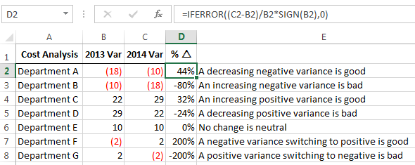
And to make sure we handle #DIV/0! errors we can wrap the formula in an IFERROR Function:
=IFERROR((C2-B2)/B2*SIGN(B2),0)
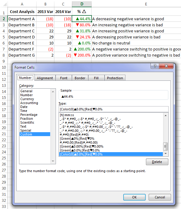
Finally we can jazz it up a bit with some Custom Number formatting to indicate the direction with both colour and a symbol:
Download the Workbook
Enter your email address below to download the sample workbook.
Thanks
Thanks to Alston for his question and to Catalin (our in-house Excel Guru), for providing this clever solution which gave me the inspiration for this post.


hello Ms Mynda, i just want to ask if there is a formula for selecting a breakdown of a certain total, for example:
A1 – 10
A2 – 80
A3 – 50
A4 – 60
A5 – 90
A6 – 100
in these data there is total of 220, how can i know the breakdown of this total from the above data, is there any formula for this? Thank you and GOD BLESS.
Hi Elinor,
I presume you’re asking for the purpose of reconciliation. If so then you can use this add-in:
https://www.summatch.com/
There is no simple formula in Excel to do this type of calculation.
kind regards,
Mynda
Thank you very much Ma’am…
One more thing I noticed is that while using the custom number formats, you can’t apply font-colour-based filters in the variance column.
Excel just doesn’t ‘recognise’ the font colours in the cells, and so, in the AutoFilter drop-down the “Filter by colour” command is disabled. 🙁
So if that’s a must for you (using font-colour-based filters), it would be better to use conditional formatting to apply the font colour, and use only the triangles in the custom number format.
Very interesting post Mynda 🙂
I have already started using it in a few workbooks where I highlight the variance figures using conditional formatting.
I also added a small tweak to the custom formatting, to make the coloured triangles aligned at the left or right edge of the cells. This helps to improve the readability of the variance figures.
For aligning them along the left edge, the custom format is:
[Color10]▲ * 0.0%” “;[Red]▼ * 0.0%” ”
For aligning them along the right edge, the custom format is:
[Color10]0.0%” “▲;[Red]0.0%” “▼
Thanks, Khushnood!
Great tip on the alignment. Thanks for sharing 🙂
My pleasure, Mynda 🙂
Thanks for sharing this Mynda. This is really helpful because it simplifies things for me. I used to create a long formulas in Excel to accomplish the improvements in negative variance… Very smart!
You’re welcome, Jyler. Glad you found it useful.
Hi Mynda,
How to enter the special symbols in the format cell ‘custom’
Hi,
How did you add the up and down triangles in the custom number formatting?
@Mark and @Karen,
To get the arrows first insert the arrow symbols into a cell (Insert tab > Symbol), then copy the symbol to the clipboard and paste it into your custom number format.
Kind regards,
Mynda
I am really interested as to how you got the delta symbols in your custom format for the cells. I searched all through the symbols lists and only found the Greek letter “delta”. Could you please demonstrate this?
Found ’em !! in Arial > Geometric Shapes. All set now.
Thanks to all. That’s a lot of sharing.
Glad you liked it, James 🙂
Hi Mynda,
Cool! Never thought of the use of SIGN for this kind of calculation. I used to put ABS to the base for calculating % change.
https://wmfexcel.wordpress.com/2013/11/30/calculating-change-is-so-easy-to-make-a-mistake/
Cheers,
Me neither, MF. We have Catalin to thank for the SIGN tip 🙂
Thanks for this post Mynda.
Always great to visit an overlooked function. I wonder if it would be useful in vba?
Just a hypothetical question: In the example you give, can anyone see a disadvantage in using Abs, as MF mentions above?
Mark
Hi Mark,
You could use SIGN in VBA but the VBA equivalent function is called SGN.
Kind regards,
Mynda