Excel PivotTable Expand, Collapse and Show Details

Excel PivotTables are a treasure trove of features. One of my favourites is the ability to expand/collapse and drill down into the data.

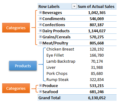
Let’s look at an example; the first column of the PivotTable below lists Categories, which group and summarise Products. We can click on the + symbols to the left of the Category name to drill down and reveal the Products within a Category:

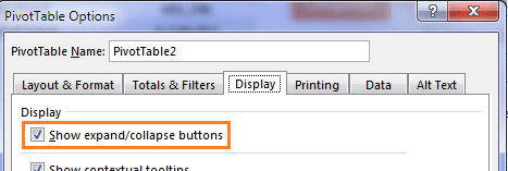
Turning On/Off Expand/Collapse Buttons

If the +/- symbols aren’t visible in your PivotTables you can turn them on in the PivotTable Options > Display tab > ‘Show expand/collapse buttons’:

PivotTable Expand/Collapse Menu

Another way to expand/collapse is to right-click the row label to reveal the Expand/Collapse menu:

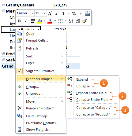
1. Choose to Expand/Collapse just one subtotal, or
2. Expand/Collapse an entire field, or
3. if you have multiple levels of row labels you can choose which level you want to expand/collapse to

Tip: Double clicking the Row labels in the PivotTable also expands/collapses one subtotal at a time.

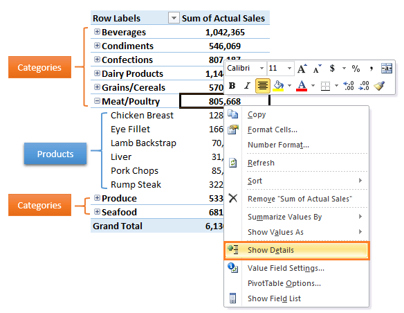
PivotTable Show Details

But what if we want to see the underlying transactions that make up the subtotals? That’s easy too. We can right-click the value (as opposed to the row label) and choose ‘Show Details’:

This will insert a new sheet with a list of all the transactions that make up the subtotal amount:

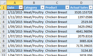
Notice how the data is already nicely formatted in an Excel Table so we can filter it if we want.

Tips:

1. Double clicking the cell containing the value you want to drill down on will also do this.
2. You can drill down from any level to extract the level detail that you want. For example double-clicking on the grand total amount will give you all of the transactions that make up the PivotTable.
3. Tip 2 is why you can go ahead and delete your original PivotTable source data, which is handy if your file is getting too big. Assuming your source data is in the same file as your PivotTable and it’s not going to change or need updating.

Group/Ungroup Selections

So far we’ve looked at the built in grouping that PivotTables automatically provide based on your source data, but you can add your own groups too.

Let’s say I wanted to group all of the meat/poultry and Seafood categories together. It’s easy:

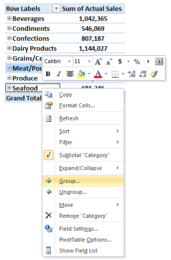
Select the rows you want in your new group > right-click > Group.

Tip: hold down the CTRL key to select non-consecutive categories. I’m going to group Meat/Poultry and Seafood:

Now you have a new group in your PivotTable called Group1:

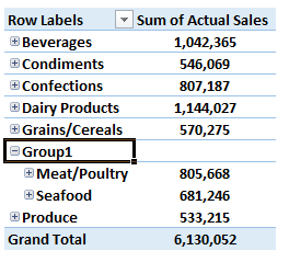
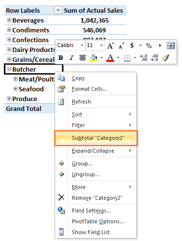
To rename it simply type over the default name ‘Group1’. I’ll call it ‘Butcher’.

If you want to display the Subtotal for your new group then right-click the row label and select ‘Subtotal…”:

Want More

If you'd like to learn more tricks like this and really master PivotTables then go ahead and join 1000's of others and check out our Xtreme PivotTable course.