Q: How do you get the PivotTable to show the missing dates in your data?
A: Not as easily as it should be, but here are a couple of workarounds you can use.
Option 1: If you don’t care how Excel formats your dates
The limitation of this option, as you will see, is that when Excel groups days in a PivotTable it shows the date formatted as “d-mmm” and you cannot change it 🙁
Note: I presume in the US it formats them as mmm-d but I cannot easily check.
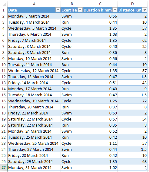
Below is my data (loosely based on Phil’s triathlon training regime!), and you can see that there are missing dates for the month of March because he doesn't train everyday:
A regular PivotTable will only display the dates present in the source data. If you want to display the missing dates for March you need to take the following convoluted steps:
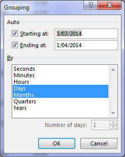
- Right-click one of the date row labels in the PivotTable > select Group > Days and Months:
- Next right-click one of the date row labels in the PivotTable > select Field Settings > Layout & Print tab > check the ‘Show items with no data’ box.
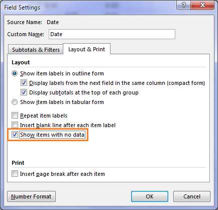
Tip: The ‘Show items with no data’ can be applied to any row label, not just dates. For example, let’s say you have data for regions A, B, C and D but B and C are not appearing in the PivotTable Report because they have no data for the filters you have applied, if you select the ‘Show items with no data’ option they will be included in the PivotTable Report with blanks/zeroes.
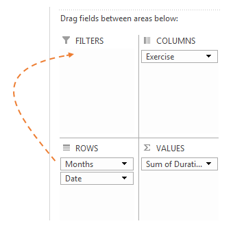
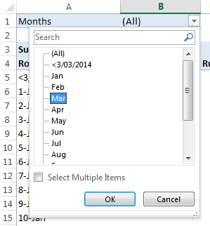
- Now your PivotTable will display every date in the year – annoying I know. To fix this drag the Months field into the Filters area of your PivotTable:
- From the Months filter select the months you want to display in your PivotTable – for me this is March.
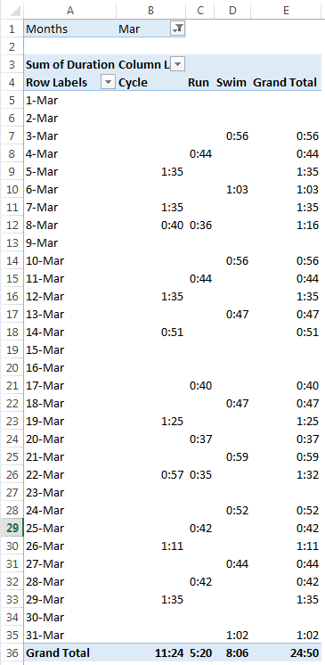
Now I have my PivotTable with the missing dates represented as I want…... well, almost – see Gripes below:
Gripes with this Method
- I can’t stipulate the range for my missing dates so I end up with a load of dates I might not want. To fix it I have to apply a workaround which are steps 3 and 4 above. I suppose it’s not that bad, but I think it could and should be better.
- My second gripe, and this is much more serious, seriously, I cannot choose how I want to format the dates in my PivotTable. I am stuck with d-mmm (if you’re in the U.S. it might be mmm-d for you), which is very annoying.
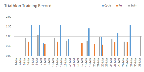
Now, depending on what you want to use the data for, it might not be that big a deal, but I want to put it into a PivotChart (which I’m not a fan of anyway as they’re too limited) and the dates are too big to fit horizontally, plus I’d like to know what day of the week I’m looking at, but I can’t so I’m stuck with a horizontal axis like this:
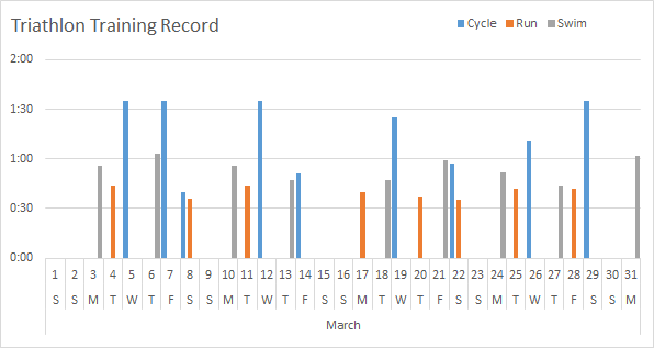
When what I want is a nice uncluttered horizontal axis more like this (a technique I teach in my Excel Dashboard course):
I know I can add columns to my source data for the day and month fields, but the point is I shouldn’t have to, damn it!
Option 2: If you want to control how Excel formats your dates
Now, since I’m fussy about how my dates are formatted I prefer this method but it’s not ideal either.
- The trick here is to add dates to your PivotTable source data for every day in the period you want, so for me I want to see every day in March 2014 represented so I’ve added dates to the bottom of my date column for every day in March using AutoFill (see rows 28:58 below):
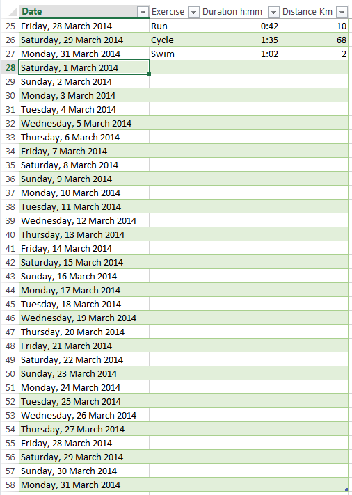
Note: You'll notice that I've added dates I already have. This is because the quickest way to add all the missing dates is to use AutoFill to create a list of dates from March 1 to 31.
It doesn’t matter that I’m repeating some dates; since they don’t have any data against these records they aren’t going to affect the values in my PivotTable Report, but they will allow me to use the ‘Show items with no data’ option without the need to Group my dates like I had to in option 1. This also means I have more options when it comes to formatting my dates.
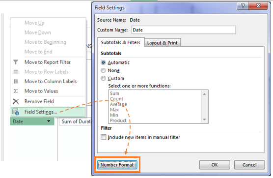
- Once you’ve built your PivotTable you can format the date row labels: in the Field list click on the down arrow beside ‘Date’ and select ‘Field Settings’, then click on the ‘Number Format’ button in the bottom left of the Field Settings dialog box:
- Choose from the default ‘Date’ formats or set your own ‘Custom’ format:

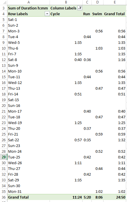
Now you have a simpler PivotTable (no filters) with dates formatted the way you want, like this:
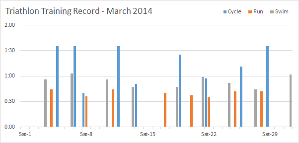
And while you still can’t get your horizontal axis like my preferred chart above (one case in point for why I don't like PivotCharts), you can change the axis label frequency to every 7 days and add tick marks for the days so it’s a bit less cluttered, although I’m not sure it’s any easier to read than the default vertical labels 🙁
[Update] Option 3 - Solve Axis Formatting Issues with a Helper Column
This technique is from Roger Govier, Microsoft Excel MVP and Consultant at Technology4U.co.uk.
Roger gets around the axis label problem with a helper column (B) in the source data. You can see in the Formula Bar below he has used the TEXT function (primarily) to create a text string comprising of the day number and first letter of the day, which is cleverly wrapped onto two lines using CHAR(10).
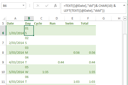
Note: Apply 'Wrap Text' format to column B of your Table if you want to see your date text string formatted as per the image above, i.e. with the date number above the letter for the day. However, this is not necessary for the PivotChart since it wraps the text because we have used the CHAR(10) character in the text string. More on that formula below.
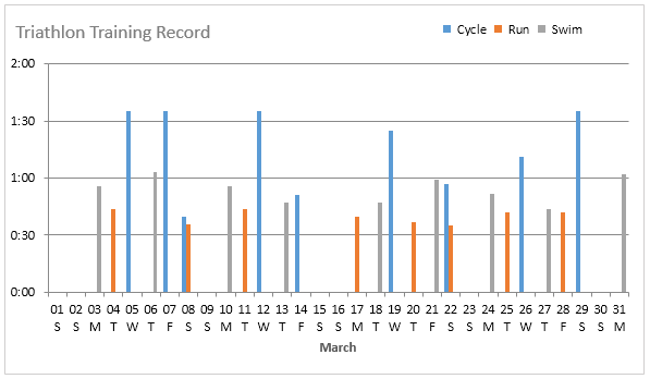
This allows us to create a chart like the one below with the horizontal axis labels formatted the way I want, AND in a PivotChart to boot:
Let's understand the components of the formula in column B:
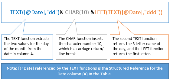
The ampersand (&) allows us to join text strings together in the one formula. More on joining text here.
More on the TEXT function here.
More on Excel Tables and Structured References here.
I'd like to say a big thank you to Roger Govier for sharing this tip.
Enter your email address below to download the sample workbook.
How to show the date? It doesn’t appear only #### show
When you see #### for a date it can mean one of two things:
1. the column isn’t wide enough to display the date. Make the column wider to fix the issue or,
2. the date is a negative value, in which case Excel can’t display negative dates since there’s no such thing. Check the formula calculating the date.
I hope that helps.
Mynda
awesome!
you saved my day bro :). It helped a lot to fill missing dates in pivot. thanks a lot.
Great to know we could help, Manish 🙂
Hello Mynda,
Thank you very much for all your very helpful resources.
I have a question closely related to this which I have not been able to fix, and suspect there is no fix to.
My data table consists of around 200 projects which all have several types of benefits (let’s simplify by saying there are three types, investment cost savings, operational cost savings, and staff cost savings). Each project has an implementation date, however some projects have no implementation date (i.e. either the date is not known or still to be determined).
I would like to have my dynamic table return a table with the sum of the savings by type (investment, operational or staff) distributed by the expected implementation date (from 2018 through 2025). For those that have an unknown or still to be determined date, I want the dynamic table to simply lump them together next to the dates with the mention, TBD or NA. Or in any case, in a separate field to those with actual dates.
Currently, as soon as there is one non-date value in the date range, the grouping of the date values per month or year disappears and I get separate date values for each data entry in the dynamic table.
I have changed all those that have TBD or No data in the date value to a fictitious value (e.g. 1/1/2040), but this is obviously sub-obtimal and delivers a dynamic table/graph representation which is not good.
Is there any solution to this? I would really appreciate it if you could give me a hand with this, as it is a really important table for my manager.
Hi Nuno,
You can’t use the built in PivotTable groupings in this instance, as you’ve found. Instead you need to add a helper column to your source data that categorizes your data into the year groupings you want. Some of these will be TBD and others will be the year (or month-year), you want to see.
Mynda
It’s unfortunate that we can’t get the first letter of the day name directly in a number format.
We can get the first letter of a month name using
=TEXT([@Date],”mmmmm”)
If you could you could simple use number formatting to produce the date format you want, without building a text string. You can get the line feed in the number format by typing Ctrl+j. It looks like you’ve just messed up the format, but it works.
You can’t enter Ctrl+j into the number format of a chart axis, but you can format the source data, and make sure the number format for the chart axis has the Linked to Source box checked to apply the format. If you then uncheck the box, you can change the number format in the worksheet dates.
Hi Jon,
I sure did have a good old rant in that post 🙂
Nice tip about CTRL+j, thanks!
You said “You can get the line feed in the number format by typing Ctrl+j. It looks like you’ve just messed up the format, but it works.”, but I’m not sure where said messed up format is that you’re referring to?
Mynda
I did tried your first Pivot Table Option 1 to change the date under Excel 2016 version. First I create a Pivot Table, Then drag Dates into Row Section, Duration h:mm to Values Section become Sum of Duration h:mm. Then drag Exercise to Column Section. Then when I use right-click on Dates’ under Group. The message told me that I cannot change that portion. Why not?? I don’t understand why I cannot from Monday ,3 March, 2014,etc to get Group under Months and Days to convert??
Hi Francis,
I’d say your dates aren’t date serial numbers that Excel PivotTables recognise and can group automatically. Tips on fixing dates formatted as text.
Mynda
In pivot Table in excel some date (15/04/2017) not showing in list.
Missing cell showing empty date but their value in other column is correct.
Hi Prakash,
Can you please upload a sample file with the problem on our forum? (create a new topic). It will be a lot easier to understand your situation and help you.
Catalin
Screen 1
21-Jun
20-Jun
29-Mar
19-Apr
7-Jul
4-Mar
17-Mar
6-Jul
27-Apr
25-May
25-May
7-Jun
21-Mar
Now go to Data Column and click ” Text to Columns”
Now change the format to Date,
6/21/2016
6/20/2016
3/29/2016
4/19/2016
7/7/2016
3/4/2016
3/17/2016
7/6/2016
4/27/2016
5/25/2016
5/25/2016
6/7/2016
3/21/2016
Hello,
I got good idea, Copy the Column ” Missing Year date column” and paste other empty column as values. Select the column, Now go to Menu Data and then click ” Text to columns” option. Problem solved. You have mm/dd/yyyy format.
Cheers
Thank you. Works like a charm! 🙂
You’re welcome, Om 🙂
Thanks for the informative post! I’m afraid, though, that there’s a bug in Excel, following your steps in option 1, in step 4, rather than picking one month try picking two, or even just choosing “Select Multiple Items” on the bottom of that menu and leaving only one month, the ENTIRE chart shows but with values only for that month!
Oooh, that does appear to be a bug. I’ll log it with MS.
Thanks for letting me know.
Mynda
Great tutorial Mynda! Thanks for sharing!
Cheers, Jon 🙂
Hi Mynda,
I use Excel 2010 and the free Power Pivot add-in, so it’s not as intuitive as Excel 2013.
In order to work, you need to pull the dates from the Calendar table and then go to the PivotTable Options, click the Display tab and check the box “Show items with no data on rows”.
Please test it, it should work.
Thanks,
Pablo
Ah, yes. Cheers Pablo. The difference is going to PivotTable Options as opposed to Field Settings as you do for a regular PivotTable.
Works perfectly. Likewise in Excel 2013 using PivotTables with multiple tables in the data model.
What a nice workaround in Option 1. Thanks for sharing!
For Option 2, I will try to avoid that as just in case user need other calculation e.g. count, it may give incorrect answer.
Cheers, MF. Glad you found it useful. For Option 2 it doens’t give incorrect answers for count/average etc. since there are no values in the Cycle, Swim or Run columns.
That’s not to say it won’t catch you out elsewhere. I haven’t tested every scenario 🙂
Kind regards,
Mynda.
Hello,
Thanks Mynda for sharing this info, it’s a great technique.
From reading the option 2, a similar solution, though a bit more complicated, is to use Power Pivot. Create a Calendar table with all the dates that you need and then establish a relationship on the dates. Finally build the pivot table from both tables.
Thanks,
Pablo
Great idea! Thanks for sharing, Pablo.
In fact you prompted me to recall that if you have Excel 2013 you can create the table and relationships without PowerPivot which would be slightly simpler.
Cheers,
Mynda.
Hi Pablo,
Actually, I don’t think you can ‘show items with no data’ in PowerPivot, so perhaps it wouldn’t work.
I haven’t tested it though.
Cheers,
Mynda.