For many years there has been something kooky going on in my Excel worksheets. It was this strange phenomenon that from time to time would rear its head.
I never had a name for it, I just knew it existed. Then one day a 3 minute video from MrExcel ended years of wonder and finally gave my ‘phenomenon’ a name.
It’s called Implicit Intersection.
Unlike the space operator which is an explicit intersection, in some situations Excel will use an implied or implicit intersection.
Let’s take a look at some examples.
Implicit Intersection Examples
Below is a list of Superheros and the number of movies made for each hero (according to Wikipedia).
Sorry, I have two boys (7 and 5) and these Superhero’s are discussed daily. So when I was thinking about what to use for my example data they were the first thing that popped in my mind! Sympathy for me will be accepted 🙂
Anyway, in column D I’ve entered the (non-array) formula =B:B+1. You can see in cell D4 that the sum is effectively B4+1, despite the fact that the formula is referencing the whole of column B.
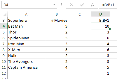
This is implicit intersection at work.
In cell D4 Excel is (in the background) converting the formula from =B:B+1 to =B4+1 because the formula is on row 4. Row 4 is implied by the location of the formula.
Equally we can see in cell D12 that the formula returns 1 because the implied cell, B12, is empty.
VLOOKUP with Implicit Intersection
The first argument of VLOOKUP, the lookup_value, can be replaced with a whole column reference and Excel will apply the implicit intersection rule (as long as your formula is in the same row as the value you're looking up):
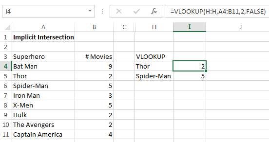
VLOOKUP using implicit intersection is the example Bill Jelen, aka MrExcel, gives in his video that ended my years of wonder.
COUNTIF to Find Duplicates
A common approach to finding duplicates is to use the COUNTIF function. Remember the syntax for COUNTIF is:
=COUNTIF(range, criteria)
You can see in the image below that the formula in cell K4 uses the same range for both the ‘range’ and ‘criteria’ arguments.
The same formula is in all cells from K4 through to K12, yet the count is different depending on which row the formula resides in.
Again, implicit intersection is at work.
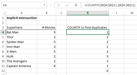
Note how cell K12 returns 0. Excel doesn’t know which cell is implicit because the formula is in a cell outside of the referenced range (B4:B11). In other words, the formula needs to be on a row within the range 4:11 for it to work.
BTW, we can tell a duplicate exists because the count is > 1.
Named Range
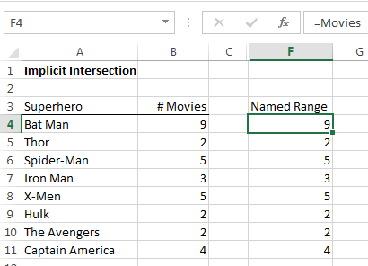
Implicit Intersection also works with Named Ranges. I’ve given cells B4:B11 the named range ‘Movies’. When we enter the same formula; =Movies, in cells F4:F11, Excel returns the results based on the implicit intersection:
Structured References
Excel Tables come with inbuilt named ranges called Structured References.
When you reference a cell in a Table from an adjacent column Excel will automatically use the Table’s structured references because implicit intersection can be employed. You can see the structured reference in the formula bar below:
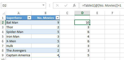
Note: If I were to tab through the cells D2:D9 you would see the same formula in every cell.
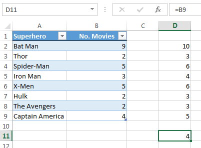
However, if you reference a cell in a table from a cell outside of the table’s rows (2:9) you will get the regular cell references, as you can see in the formula bar below for cell D11:
Array Formulas
Sometimes when you enter an array formula and forget to press CTRL+SHIFT+ENTER you will still get a result as opposed to an error.
This is typically implicit intersection at work. For example, let’s take the array formula below that hasn’t been entered with CTRL+SHIFT+ENTER:
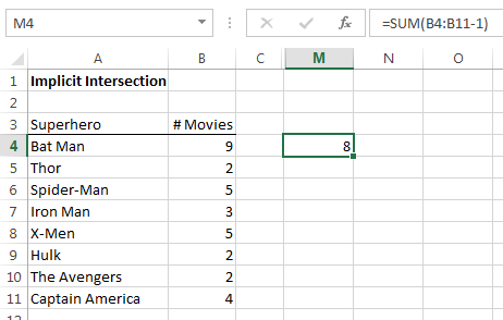
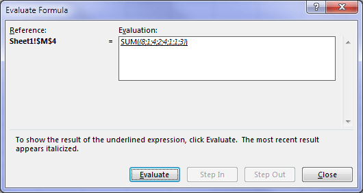
We can see that it is actually calculating =SUM(9-1), whereas if entered correctly with CTRL+SHIFT+ENTER you would get 24:
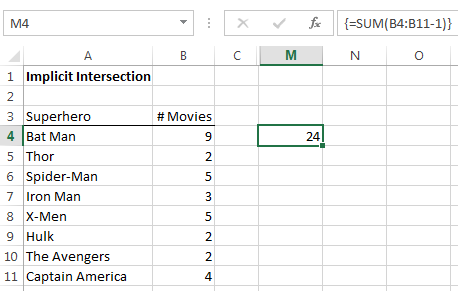
We can see below in the Evaluate Formula window that when correctly entered the array formula takes a 1 off each value in column B, then adds them up:
Enter your email address below to download the sample workbook.
Other Uses
Now, I’m not recommending you use whole column references, or even the implicit intersection willy nilly as I think it has the potential to confuse other users.
The reason I’ve written about it is to raise awareness and prevent you from going through years of wondering like I did.
What can I say….I’m nice like that 😉
The best practical use for implicit intersection I can think of is to use it with named ranges in formulas to make the formula easier to read and write. i.e. in the same way structured references work in Excel Tables.
Have you got a practical use for Implicit Intersection? Please share it in the comments below.
Thanks
I'd like to thank MrExcel (Bill Jelen) for ending years of wonder about these strange goings on in my Excel worksheets. I can once again sleep at night!
I’ve been using some of these for years not knowing it was a thing, but most I’d never really considered. It is amazing how much is buried in Excel.
I sometimes wonder if the developers for Excel today have knowledge of *everything* in the product or have just left some code untouched for years.
Indeed it is amazing how much is burried in Excel. And I’m sure today’s developers don’t know everything about what is burried in Excel. It has, litterally, millions of lines of code, which is also why changes can take a long time to implement.
I’m a bit late to this thread but I found it very helpful, and I think others will too. I’d like to point out another impact of implicit intersection.
Our loading dock people had a request for us to write a formula to check the status of packages in transit. When a package is shipped they received a (say) 14-digit tracking number. The company would send a daily sheet showing where packages were, but their tracking info was 24-digits with the 14-digit segment buried in the 24-digit number, not always at the same place. They could manually execute a FIND for each row, but they wanted a formula they could copy down to say whether or not their package was in the mix, and what the associated status was.
We wrote an array formula with FIND() to say if the number existed, and use IFERROR() or ISERR() to say “No” in the field if the answer wasn’t numeric (since FIND returns an error if it can’t find the value). However, for returning the status we used INDEX/MATCH equivalents, and the FALSE return for a negative FIND ends up giving a zero for the INDEX row. Of course, INDEX interprets a 0 as returning the entire row of the array. So with our formula in each cell next to the original 14-digit tracking number, INDEX would return the array row of the status result set based on implicit intersection rather than “Not there” result it should have returned.
Hi GMF,
Interesting gotcha with INDEX interpretting 0 and then implicit intersection being applied. Thanks for sharing.
Mynda
Hi Mynda,
Thank you for this informative and comprehensive post about Implicit Intersection. It’s really a great post! Clear explanation and nice visuals.
Imagine all of the errors that exist because people forget to press Control Shift Enter for an array formula. They see a non error numerical value and think that it’s correct.
Cheers,
Kevin Lehrbass
https://www.youtube.com/user/MySpreadsheetLab
Hi Kevin,
It’s nice to have you drop by. Glad you enjoyed my tutorial 🙂
Mynda
I am having a difficult time getting Excel 2007, Protect worksheet and Protect workbook to work properly. Is there some tips or oddities that might help me out? It seems as though it will save the file with a password protected worksheet, but, won’t ask for the password to unprotect the worksheet.
I have been trying to set up a macro that will password protect each worksheet as well as password protect the workbook but so far I have not been successful in getting this to work. I was planning on setting up a second macro to unprotect all tabs so that we can enter data for a new month, then reprotect the tabs and the file. I have been using Excel for some time now, but this version of Excel has me stumped!! Any advice you can offer is greatly appreciated. Thanks.
Hi Carol,
If you upload a sample of your workbook, with your code, that was very useful.
Have you tried to set a password? Seems that you are protecting sheets without password, like:
Sheets("Sheet1").ProtectIf so, use code like this:
Sheets("Sheet1").Protect Password:="Pass", DrawingObjects:=False, Contents:=True, Scenarios:=False, AllowFormattingRows:=TrueIf you need more help, please use Help Desk: https://www.myonlinetraininghub.com/helpdesk/ to upload your file, and describe what you are trying to achieve.
Thank you,
Catalin
Wow. This is something I’ve never heard of. It feels like this is some sort of hidden gem in Excel. Thanks for sharing, Mynda!
🙂 You’re welcome, Joseph. Glad you liked it.
Very interesting phenomena here Mynda! I read through your ‘space’ and ‘implicit’ intersection articles and am still trying to grasp the practical uses of both features.
I understand the simplicity with using implicit intersection with named ranges, but when it comes to readability and debugging formulas, I just don’t see the usefulness of these features.
I’m really curious to see if anyone has come up with a really good use case for these features. They seem like such simple ways to access ranges of data but the difficulty in reading them in the formula bar (and understanding how they work) would prevent me from actively using them in my worksheets.
Thanks, KeyCuts. I agree with you. I think if a function can’t handle an array it should return an error (unless entered as an array formula), with the exception of Structured References which look different and therefore a different result is reasonable….maybe I’d extend this to named ranges too, but a regular range, no.
Implicit intersection is mysterious thing indeed 🙂
I have read excellent explanation of this few months ago in Mike Girvin’s book “CTRL+SHIFT+ENTER Mastering Excel array formulas”
Hi Pmsocho,
Yes, Mike Girvin’s book is excellent. Can’t say I remember the part on Implicit Intersection though…but then I haven’t finished the book yet so maybe I haven’t got to it!
Cheers,
Mynda.
It was in one of the first chapters.
Not as comprehensive and detailed as yours but enough to understand how it works 🙂
🙂 ha, I don’t remember it, but then I did skim read a lot of it! That’ll teach me.
Amazing how sometimes only hearing the right words & terms helps us understanding the phenomena we knew already. That’s why I, as well, tend to be as descriptive as possible. (Or should I say ‘plastic’?) Because, at the end of the definition -it’s only a matter of perspective, isn’t it? – some of them work better than the others by giving you a ‘bigger picture’, but the whole ‘story’ actually should always be valued over the individual ‘chapters’, alone, I’d say.
My preferred scenario (in explaining to myself this) would involve “vector-scalar dichotomy” – a single value (single cell) always ‘sees’ the corresponding (single) value from a stack; i.e. whenever the formula was entered as usual, with ENTER, by which we imply that the ranges should treated as singles (aka scalars).
As of practical example…
Not so sure how practical is it but the one that comes to mind is with exact match in MATCH(): for detecting actual row number where our data seats. Normally, we should have know the beginning of the list, is it named, what column exactly etc. Actually the exact column is all we need: we can just check against the whole say H:H and it should work fine. (Assuming that we wouldn’t name the list by its member, and that we don’t hold multiple instances there neither.)
Thanks, Zoran 🙂
With your MATCH example do you mean like this:
Cheers,
Mynda.
For example, yes, only columns from two sheets would appear little bit more practical. 😀 Should that matter at all.. 😀
I’m not following you 🙁
Sorry, I thought for the two columns (A:A), that it would be a little bit more practical if the one of them referring @Any other Worksheet. (Instead of looking within the same. Although it wouldn’t change thing as for the example.)
Oh, I see 🙂