Last week Ann emailed me a question and before I had a chance to even look at it she emailed me again with her solution. I like those kind of questions 😉
This is something I’ve never seen before and it’s quite clever so I thought I’d share it with you.
Q: How can I sum data in column C for all names in column B beginning with A, B and C?
A: =SUMIF(B2:B13,"<D*",C2:C13)
I never knew you could use greater than or less than operators with letters!
I had a play around with this technique and there are a couple of quirks with it.
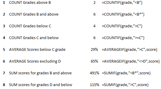
I’ve set up some mock data below which I'll use in my examples.

Note: The Grade range B2:B13 has a named range ‘grade’ and the Score range C2:C13 has a named range ‘score’ which you will see in my formulas below:
More Examples
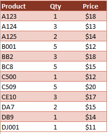
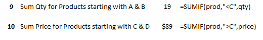
Using the table below we want to sum various columns filtering on the first letter of the product code.
Note: Again I have named the Product range 'prod', the Qty range 'qty' and the Price range 'price'.
Initially I expected to need to use the wildcard symbol * to ignore the remaining characters in the product code, as Ann did in her answer, but it turns out you don't need to.
The formulas below calculate correctly without the need for the wildcard.
Quirks
In formula number 2 the criteria includes a wildcard “<B*”. This wildcard results in Excel counting both B and A grades.
However if you try to use the wildcard with a greater than operator like this “>B*” it only counts grades from C onward and excludes B. Strange huh?
UPDATE: click here to understand why wildcards work differently when testing strings using > or <.
Hi Mynda,
i’m back with question to you!!
How to get sum of unique text within the same column where the names are repeated more than 6-10 times. But i need to only unique… This result need only by using formulas
Eg: A,B,C,A,B,E,G,E,F,G,A,B,E,D then unique count is 7 in single cell
Thanks,
Ramu
Hi Ramu,
You need an interim step before getting your single value of 7, which you can find here:
https://www.myonlinetraininghub.com/excel-pivottables-unique-count-3-ways
I’m not aware of any way to do this in one cell only.
Mynda
Hi Ramu,
You can try the FREQUENCY formula:
=SUM(IF(FREQUENCY(MATCH(A1:A14,A1:A14,0),MATCH(A1:A14,A1:A14,0))>0,1))
Or a countif:
=SUM(1/COUNTIF(A1:A14,A1:A14)) (this is an array formula, press Ctrl+Shift+Enter after editing the formula)
Catalin
Ah,ha. Genius, Catalin. I should have left this one to you 🙂
This is a quick post to provide some detail on using the wildcard search for WMIC . This feature of the command structure will allow you to use like conditions in a where clause to look for objects that match a specific pattern. For those of you comfortable with the SQL syntax for the same task, this will be quite familiar.
Hi Socorro Franco,
We will surely be glad to have that one here.
Thanks.
CarloE
Hello Mam,
From past 3 months, I’m try to find out calculation behind Icons in Conditional formatiing. My question is how does icons is determined “Green >=67%”, “Amber 33%”, & “Red <33%" indication in when we use default Icons/Bars/colour scales..
I will be thankful to you, if you can send me or share the mechanisim used by Microsoft to determine those icons by default.
Thanks and Wish you Happy New Year!!
Ramu
India (Bangalore)
Hi Ramu,
Microsoft MVP Tushar Mehta explains it best here where he says:
“From some preliminary tests it appears the thresholds are calcuated as % * (max – min) + min
Suppose you have a 3 icon set (red, yellow, green), 2 thresholds at 33% and 67%, and the data range from 1 to 14. Then, the yellow icon will show for a value that is at least 33% *(14 – 1) +1 or 5.29 (and of course, less than the green threshold). Similarly, the green icon shows for a value that is at least 67% * (14 – 1) +1 or 9.71”
Kind regards,
Mynda.
when comparing two strings with the wildcards are normal characters … then the text is “B*”>”B” in the same manner of which is “Ba” or “Baaa” or B from any other character after
best regards
r
I left a comment but I think I have not explained well 🙂
what I mean is that when we use operators between strings, wildcards are not considered special characters, but simply as text … so B * B is considered to be followed by the character * (code 42)
ciao
r
Thanks, Roberto.
John Edwards emailed me last week and explained it this way:
“The equation is saying “>BZZZZZZ…” when you substitute the highest possible value for the wildcard “*” and therefor C is the next available number.
When you use “<B*” then when you substitute the wild card for the next available value it would be “<BA” which is “B” ”
Mynda.
is not so … try with this greater than:
B)
B+
B
countif(range;”>B*”) return 1 … only B+ is > of B* because
character code(“+”) ->43
character code (“)”) -> 41
character code (“*”) -> 42
when we use operators <> between strings, wildcards are not considered special characters, but simply as text … so B * B is considered to be followed by the character * (code 42)
regards
r
Thanks Ann and Mynda, I enjoyed reading.
Although I was aware of various operators inside COUNTIF, this is new use of it and I like it.
The other, very useful, could be for sorting text. For example, chandoo.org wrote about it.
Cheers!
🙂 Cheers, Zoran.
thanks Ann